About Decision Tree
Decision Tree is a kind of common classification and regression algorithm in machine learning, although it's a basic method, some advanced learning algorithms such as GBDT (Gradient Boosting Decision Tree) are established on it. There are approximate three steps in decision tree learning: feature selection, decision tree generating and decision tree pruning. In the essence, decision tree splits the data set according to the information gain, which means this algorithm chooses the features which can make the data set has the minimum uncertainty in each steps. In this blog, I'm going to introduce the feature selection, decision tree generating and decision tree pruning respectively, and the classification and regression tree (CART) will be detailedly interpreted.
All the codes in this atricle are collected on my github: Decision Tree
Feature Selection
We need a calculation method or regulation to mark each features in the data set since the essence of decision tree learning is splitting the data set based on features, in other word, we need to determine which feature will be the 'hero' or the 'entrance' in the next level of the decision tree. Therefore, we need to calculate the information gain for the current data set.
Entropy and Conditional Entropy
For better understanding the information gain, we need to know the concept of entropy first. The entropy is defined as 'a metric can represent the uncertainty of random variable' , assume \(X\) is a random variable, such that the probability distribution is: \[P(X=x_i) = p_i, (i=1,2,3,...,n)\] And the entropy of \(X\) is: \[H(p) = -\sum_{i=1}^n p_i * log(p_i)\] A large entropy represents a large uncertainty, and the range of \(H(p)\) is: \[0 \leq H(p) \leq log(n)\] If we assume there is a random variable \((X,Y)\), and the union probability distribution is: \[P(X=x_i, Y=y_j) = p_{ij}, (i=1,2,...,n; j=1,2,...,m)\] And the conditional entropy is: \[H(Y|X) = \sum_{i=1}^n p_i * H(Y|X=x_i)\] Which represents the uncertainty of random variable \(Y\) with the given random variable \(X\). In this situation, we call entropy and the conditional entropy as empirical entropy and empirical conditional entropy.
Information Gain
Concept of Information Gain
Now we can learn what is information gain. As the definition, 'information gain represents the degree of reduction of the uncertainty of class \(Y\) by giving the feature \(X\)'. Here we use \(D\) to denote the data set, and \(A\) to denote the specific feature, and the information gain of feature \(A\) for data set \(D\) is the difference of empirical entropy and empirical conditional entropy: \[g(D, A) = H(D) - H(D|A)\] We can easily know that different features always have different information gain, a feature with large information has strong ability on classification.
Process of Calculating Information Gain
calculate the empirical entropy \(H(D)\): \[H(D) = -\sum_{k=1}^K {|C_k|\over |D|} * log_2{|C_k|\over |D|}\]
calculate the empirical conditional entropy of feature \(A\): \[H(D|A) =\sum_{i=1}^n {|D_i|\over |D|} * H(D_i)=-\sum_{i=1}^n {|D_i|\over |D|} * \sum_{k=1}^K {|D_{ik}|\over |D_i|} * log_2{|D_{ik}|\over |D_i|}\]
calculate the information gain: \[g(D, A) = H(D) - H(D|A)\] Where:
\(C_k\) represents the classes, \(|C_k|\) is the amount of class \(C_k\), and \(\sum_{k=1}^K|C_k|=|D|\);
\(D_i\) represents the subsets which are splitted according to the feature \(A\), and \(\sum_{i=1}^i|D_i|=|D|\);
\(D_{ik}\) represents the subset which all the elements are belong to the class \(C_k\) in the subset \(D_i\)
Information Gain Ratio
Since splitting the data set by using information gain approach may tends to select the features with more values in some situations, we can use another method named information gain ratio to solve this problem. Information gain ratio, as its name, is the ratio of the information gain and empirical entropy: \[g_R(D,A) = {g(D,A) \over H_A(D)}\]
Decision Tree Generation
I'm going to introduce two decision tree generating algorithms which are ID3 and C4.5, the former method will be mainly introduced. In addition, the process of generation and pruning of CART will be explained in the next part.
ID3 Algorithm
ID3 algorithm splits the data set by using the features which have the largest information gain value, and generate the decision tree recursively. The process of the algorithm is:
Steps
Setting \(T\) as the leaf node and use\(C_k\) as the class label if all the distances in subset \(D\) are belong to class \(C_k\), return \(T\);
If there is no further features meet the requirement (the value of information gain less than the threshold), setting \(T\) as the leaf node and use the class of most distances as label, return \(T\);
Otherwise, calculating the information gain values of each features for data set \(D\), choosing the largest one as \(A_g\) which will be the splitting point;
For each possible values (\(a_i\)) in \(A_g\), splitting the data set into plenty of subsets \(D_i\) by \(A_g = a_i\), use the class of most distances in each subset \(D_i\) as labels, return \(T\);
For each sub-nodes in step 4, use \(D_i\) as training set, \(A-A_g\) as feature set, execute the step 1 to 4 recursively until meet the stopping conditions, return \(T_i\)
Code
Import the necessary third-party libraries : 1
2
3
4
5
6
7
8
9
10
11
12
13
14import numpy as np
import pandas as pd
import matplotlib.pyplot as plt
%matplotlib inline
from sklearn.datasets import load_iris
from sklearn.model_selection import train_test_split
from collections import Counter
import math
from math import log
import sys
import pprint
First we calculate the information gain value : 1
2
3
4
5
6
7
8
9
10
11
12
13
14
15
16
17
18
19
20
21
22
23
24
25
26
27
28
29
30
31
32
33
34
35
36
37
38
39
40
41
42
43
44
45
46
47# empirical entropy
def cal_entropy(self, datasets):
n = len(datasets)
label_count = {}
# get distribution(Pi)
for i in range(n):
label = datasets[i][-1]
if label not in label_count:
label_count[label] = 0
label_count[label] += 1
empirical_entropy = -sum([(p/n) * log(p/n, 2) for p in label_count.values()])
return empirical_entropy
# empirical conditional entropy
def cal_conditional_entropy(self, datasets, axis=0):
n = len(datasets)
feature_sets = {}
for i in range(n):
feature = datasets[i][axis]
if feature not in feature_sets:
feature_sets[feature] = []
feature_sets[feature].append(datasets[i])
empirical_conditional_entropy = sum([(len(p)/n) * self.cal_entropy(p)
for p in feature_sets.values()])
return empirical_conditional_entropy
# calculate the difference between two entropy
def info_gain(self, entropy, con_entropy):
return entropy - con_entropy
# calculate information gain
def get_info_gain(self, datasets):
feature_count = len(datasets[0]) - 1
empirical_entropy = self.cal_entropy(datasets)
best_feature = []
for c in range(feature_count):
c_info_gain = self.info_gain(empirical_entropy,
self.cal_conditional_entropy(datasets, axis=c))
best_feature.append((c, c_info_gain))
best = max(best_feature, key=lambda x : x[-1])
# best : ((feature_id, feature_info_gain))
return best
Define the class Node as : 1
2
3
4
5
6
7
8
9
10
11
12class Node:
def __init__(self, splitting_feature_id=None, class_label=None, data=None,
splitting_feature_value=None):
self.splitting_feature_id = splitting_feature_id # splitting feature
self.splitting_feature_value = splitting_feature_value # splitting feature value
self.class_label = class_label # class label, only leaf has
self.data = data # labels of samples, only leaf has
self.child = [] # child node
def add_node(self, node):
self.child.append(node)
Then achieve the ID3 algorithm : 1
2
3
4
5
6
7
8
9
10
11
12
13
14
15
16
17
18
19
20
21
22
23
24
25
26
27
28
29
30
31
32
33
34
35
36
37
38
39
40
41
42def train(self, train_data, node):
_ = train_data.iloc[:, :-1]
y_train = train_data.iloc[:, -1]
features = train_data.columns[:-1]
# 1. if all the data in D belong to the same class C,
# set T as single node and use C as the label, return T
if len(y_train.value_counts()) == 1:
node.class_label = y_train.iloc[0]
node.data = y_train
return
# 2. if feature A is empty, set T as single node and use the label,
# most C as the label, return T
if len(features) == 0:
node.class_label = y_train.value_counts().sort_values(ascending=False).index[0]
node.data = y_train
return
# 3. calculate the largest inforamtion gain, use Ag to represents the best feature
max_feature_id, max_info_gain = self.get_info_gain(np.array(train_data))
max_feature_name = features[max_feature_id]
# 4. if the information gain is smaller than threshold, set T as single node,
# and use the most C as the label, return T
if max_info_gain <= self.epsilon:
node.class_label = y_train.value_counts().sort_values(ascending=False).index[0]
node.data = y_train
return
# 5. splitting D according to each possible values in the feature A
feature_list = train_data[max_feature_name].value_counts().index
for Di in feature_list:
node.splitting_feature_id = max_feature_id
child = Node(splitting_feature_value = Di)
node.add_node(child)
sub_train_data = pd.DataFrame([list(i) for i in train_data.values if i[max_feature_id] == Di],
columns = train_data.columns)
# 6. create tree recursively
self.train(sub_train_data, child)
C4.5 Algorithm
The C4.5 algorithm becomes extremely easy to understand after introducing the ID3 algorithm, cause there's only one different point between the two methods, that is C4.5 algorithm uses information gain ratio to choose the splitting feature instead of using information gain, besides this, other steps in C4.5 are same with those in ID3 algorithm.
Decision Tree Pruning
A Simple Pruning approach
In this part, we just discuss the pruning algorithm for ID3 and C4.5, the pruning for CART will be interpreted in the next part.
We have discussed the decision tree generating approached in the above part, however, it can overfit easily if there're lots of levels in the decision tree, so we need to prune the tree to avoid overfitting and simplify the process of calculating. Specifically, we cut some leaf nodes or sub-tree from the original tree and use their parents nodes as the new leaf nodes.
Like the other machine learning algorithms, here we prune the decision tree by minimising the loss function. Assume that \(|T|\) is the number of leaf nodes, \(t\) represents the leaf nodes and there are \(N_t\) samples in it, use \(N_{tk}\) to denote the number of samples which belong to class \(k\) in \(N_t\), where \(k=1,2,...,K\) ; \(H_t(T)\) is the empirical entropy of leaf node \(t\), then define the loss function as : \[C_\alpha(T) = \sum_{t=1}^{|T|}N_t*H_t(T) + \alpha|T|\] We define the training error as : \[C(T) = \sum_{t=1}^{|T|}N_t*H_t(T) = -\sum_{t=1}^{|T|}\sum_{k=1}^KN_{tk} * log {N_{tk}\over N_t}\] In the above formula, the term \(|T|\) which the number of leaf nodes, can represent the complexity of decision tree, the parameter \(\alpha\), can be understood as the coefficient of regularization, so the term \(\alpha|T|\) actually has the same function with regularization term, which can find the trade-off between the complexity and precision of model. A larger \(\alpha\) can promote to choose a simple model and a smaller \(\alpha\) promote to choose a complex model.
Our pruning algorithm is going to find the sub-tree with the minimum loss function, here we calculate the loss value \(C_\alpha(T)\) for the current tree, then calculating it again after cutting the brunch (sub-tree) or leaf node, now we get two different information gain values, record as \(C_\alpha(T_B)\) and \(C_\alpha(T_A)\), so we can determine whether it's worth to cut this brunch or not by comparing the two error values, the specific steps are :
Calculating the empirical entropy for each leaf nodes;
Going back to the parents nodes recursively, cutting the brunch and comparing the error values between before cutting and after cutting, if \(C_\alpha(T_A) \leq C_\alpha(T_B)\), saving the pruning action and setting the parent node as the new leaf node, otherwise, recover the original tree;
Repeating the step 2 until all the nodes have been checked, then get the sub-tree with the minimum loss function
Code
First, we need to achieve the loss function which is the \(C_\alpha(T)\) in the above formula : 1
2
3
4
5
6
7
8
9
10
11
12
13
14
15
16
17
18
19
20
21
22
23
24
25
26
27
28
29
30
31
32# calculate C_alpha_T for current sub-tree
def c_error(self):
leaf = []
self.find_leaf(self.tree, leaf)
# count the N_t, len(leaf_num) == |T|
leaf_num = [len(l) for l in leaf]
# calculate empirical entropy for each leaf nodes
entropy = [self.cal_entropy(l) for l in leaf]
# alpha * |T|
alpha_T = self.alpha * len(leaf_num)
error = 0
C_alpha_T = 0 + alpha_T
for Nt, Ht in zip(leaf_num, entropy):
C_T = Nt * Ht
error += C_T
C_alpha_T += error
return C_alpha_T
# find all leaf nodes
def find_leaf(self, node, leaf):
for t in node.child:
if t.class_label is not None:
leaf.append(t.data)
else:
for c in node.child:
self.find_leaf(c, leaf)
Then calculate loss value for the original tree, starting pruning : 1
2
3
4
5
6
7def pruning(self, alpha=0):
if alpha:
self.alpha = alpha
error_min = self.c_error()
self.find_parent(self.tree, error_min)
In which the find_parent function corresponds the step 2 in the above principle introduction part : 1
2
3
4
5
6
7
8
9
10
11
12
13
14
15
16
17
18
19
20
21
22
23
24
25
26
27
28
29
30
31
32
33
34
35
36
37
38
39
40
41
42
43
44
45
46
47
48
49
50
51
52
53
54
55
56
57
58
59
60
61
62
63
64
65
66
67
68
69
70def find_parent(self, node, error_min):
'''
leaf nodes : class_label -> not None
data -> not None
splitting_feature_id -> None
splitting_feature_value -> None
child -> None
---------------------------------------------
other nodes: class_label -> None
data -> None
splitting_feature_id -> not None
splitting_feature_value -> not None(except root)
child -> not None
'''
# if not the leaf nodes
if node.splitting_feature_id is not None:
# collect class_labels from child nodes
class_label = [c.class_label for c in node.child]
# if all the child nodes are leaf nodes
if None not in class_label:
# collect data from child nodes
child_data = []
for c in node.child:
for d in list(c.data):
child_data.append(d)
child_counter = Counter(child_data)
# copy the old node
old_child = node.child
old_splitting_feature_id = node.splitting_feature_id
old_class_label = node.class_label
old_data = node.data
# pruning
node.splitting_feature_id = None
node.class_label = child_counter.most_common(1)[0][0]
node.data = child_data
error_after_pruning = self.c_error()
# if error_after_pruning <= error_min, it is worth to pruning
if error_after_pruning <= error_min:
error_min = error_after_pruning
return 1
# if not, recover the previous tree
else:
node.child = old_child
node.splitting_feature_id = old_splitting_feature_id
node.class_label = old_class_label
node.data = old_data
# if not all the child nodes are leaf nodes
else:
re = 0
i = 0
while i < len(node.child):
# if the pruning action happend,
# rescan the sub-tree since some new leaf nodes are created
if_re = self.find_parent(node.child[i], error_min)
if if_re == 1:
re = 1
elif if_re == 2:
i -= 1
i += 1
if re:
return 2
return 0
CART
As the name of this algorithm -- classification and regression tree, it can apply on both classification and regression, actually the essence of regression tree is based on classification principle, I'm going to explain it later.
Regression Tree
Principle of Generating
The process of generating regression tree is also the procedure of establishing binary decision tree recursively by minimising the mean square error.
In the regression problems, we assume the output \(Y\) is continuous variable, so the training set is : \[D = \{(x_1,y_1),(x_2,y_2),...,(x_n,y_n)\}\] Assume that we have splitted the data set into \(M\) units: \(R_1, R2,...,R_M\) , and there are one unique output value in each units \(R_m\), record as \(c_m\), in other word, we split the training set into plenty of units, and calculate an output or prediction value for each subsets, therefore, the model can be represented as : \[f(x) = \sum_{m=1}^Mc_m\] And we use the mean square error to evaluate the training error for our model : \[\sum(y_i-f(x_i))^2\] In addition, the optimal output value of \(R_m\) is : \[c_m = average(y_i|x_i \in R_m)\] Now, we need to choose the appropriate feature and value to split the data set, we call the chosen feature as splitting variable and the value is splitting point. Actually there's no sample or convenient method to find these two value, what we can do is go through all the features and for possible values of each features, calculate the summary error of the two subsets (units) which are splitted based on the values. The detailed steps are:
For the all features, scan possible values, find the specific feature \(j\) and value \(s\) which can guarantee the below formula reaches at the minimum value : \[\min_{j,s} \{ \min_{c_1}\sum_{x_i\in R_1}(y_i-c_1)^2 + \min_{c_2}\sum_{x_i\in R_2}(y_i-c_2)^2 \}\]
For the specific \((j,s)\), splitting the data set and calculate the outputs : \[R_1(j,s)=\{x|x^{(j)}\leq s\}, R_2(j,s)=\{x|x^{(j)}\geq s\}\] \[c_m={1 \over N_m} * \sum_{x_i\in R_m}y_i, (x\in R_m, m=1,2)\]
Repeat the first two steps recursively, until the deep of level reaches at the previous setting
Then we can get the decision tree model : \[f(x) = \sum_{m=1}^Mc_m\]
Code
First, we define the Node class for the tree as : 1
2
3
4
5
6
7
8
9
10
11
12
13
14
15
16
17
18
19
20class Node:
def __init__(self, splitting_name=None, splitting_value=None, c=None):
'''
leaf : splitting_name --> None
splitting_value --> None
child --> None
c --> Not None
-------------------------------
others: splitting_name --> Not None
splitting_value --> Not None
child --> Not None
c --> Not None
'''
self.splitting_name = splitting_name
self.splitting_value = splitting_value
self.child = []
self.c = c
def add_node(self, node):
self.child.append(node)
The mean square error method and the optimal \(c_m\) calculation : 1
2
3
4
5
6
7
8
9
10
11
12def mse(self, r, c):
y = np.array(r['target'])
error = 0
for i in y:
error += np.power((i - c), 2)
return error
def get_best_c(self, r):
# target is the label feature
y = r['target']
return np.mean(y)
As for the training part, achieving the above first two steps recursively : 1
2
3
4
5
6
7
8
9
10
11
12
13
14
15
16
17
18
19
20
21
22
23
24
25
26
27
28
29
30
31
32
33
34
35
36
37
38
39
40
41
42
43
44
45
46
47
48
49
50
51
52
53
54
55
56
57
58
59
60
61
62def train(self, dataset, node, max_depth, depth):
'''
@ dataset: the training data
@ node: nodes of the tree
@ max_depth: the total deep of the tree
@ depth: current depth
'''
train_data = dataset.iloc[:, 0:-1]
# if the data set can't be splitted, return
if train_data.shape[0] == 0:
return
# create two child nodes for each non-leaf nodes
child1 = Node()
child2 = Node()
node.add_node(child1)
node.add_node(child2)
# initial the error as infinity
error_sum = float('inf')
# go through the features' values, find the j,s
for feature_name in train_data.columns.values:
for feature_value in train_data[feature_name]:
# split the data set into two units
r1_list = [rows for index, rows in dataset.iterrows()
if rows[feature_name] < feature_value]
r2_list = [rows for index, rows in dataset.iterrows()
if rows[feature_name] >= feature_value]
r1 = pd.DataFrame(r1_list, columns=dataset.columns)
c1 = self.get_best_c(r1)
error1 = self.mse(r1, c1)
r2 = pd.DataFrame(r2_list, columns=dataset.columns)
c2 = self.get_best_c(r2)
error2 = self.mse(r2, c2)
if (error1 + error2) < error_sum:
error_sum = error1 + error2
node.splitting_name = feature_name
node.splitting_value = feature_value
child1.c = c1
child2.c = c2
print(depth, node.splitting_name, node.splitting_value)
# delete the splitting variable
r1 = r1.drop(node.splitting_name, axis=1)
r2 = r2.drop(node.splitting_name, axis=1)
# if has arrived at the last level, return
if depth == max_depth:
return
# repeat the above actions for each childs
self.train(r1, child1, max_depth, depth+1)
self.train(r2, child2, max_depth, depth+1)
return
The Idea of Classification
As we said, the essence of regression tree is based on the idea of classification principle, and now I'm going to give the interpretation.
In the above part, we mentioned that using the average value of the labels as the output in each subsets (units) which means we seem the each units as a 'class', and the class label is the output \(c_m\). When we need to predict for a new data item, the model just need to classify it according to the splitting variable and splitting point which we found previously, therefore, when the model classify the data into a leaf node, the output \(c_m\) of that leaf node is our prediction value.
Here we use a graph to help us to understand it better : 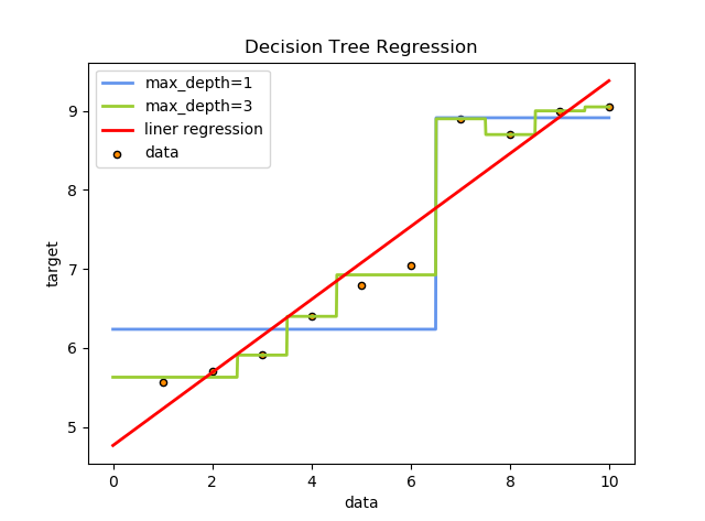
As we see, when the max_depth is equal to 1, the data is approximately splitted into two parts, and be classified into more classes when the value of max_depth is 3. Therefore, in fact, the regression tree use the idea of classification to classify the 'similar' samples as a specific class, and use the average value of their labels as the class label, in this way a regression model has achieved.
Classification Tree
Generating Principle
The core concept of generating of classification tree is using the Gini Index to select the optimal features and determine the optimal the binary value splitting point in each levels.
Assume that we have \(K\) classes in total, and the probability of sample belongs to the class \(k\) is \(p_k\), so that the Gini Index can be defined as : \[Gini(p) = \sum_{k=1}^K p_k * (1-p_k) = 1 - \sum_{k=1}^K p_k^2\] And for the binary classification problem, we have : \[Gini(p) = 2p * (1-p)\] For a given data set \(D\), there has : \[Gini(D) = 1 - \sum_{k=1}^K ({|C_k| \over |D|})^2\] In which \(C_k\) is the subset of \(D\) which the samples belong to the class \(k\), and \(K\) represents the number of classes.
If we split the data set into two parts \(D_1\) and \(D_2\) according to whether the value of feature \(A\) is equal to the possible value \(a\), then the gini index in this situation is : \[Gini(D,A) = {|D_1|\over |D|} * Gini(D_1) + {|D_2|\over |D|} * Gini(D_2)\] Where like the entropy, gini index can also represent the uncertainty of data set, and \(Gini(D,A)\) represents the uncertainty of data set which is splitted by \(A=a\), in addition, still like the entropy, a large gini index value means the large uncertainty.
The below steps show the detailed process of classification tree generating :
For each feature \(A\), and for its each possible value \(a\), splitting the data set \(D\) into two parts \(D_1\) and \(D_2\) according to whether \(A=a\), calculate the value of \(Gini(D, A)\);
For each feature and its possible value, select the optimal feature \(A\) and the splitting point \(a\) which can make \(Gini(D, A)\) has the minimum value, and distribute data set to \(D_1\) and \(D_2\) respectively;
For the sub-nodes, repeat the first two steps recursively until there's no further features or reaches at the max depth, or the number of samples in node is less than the threshold which we set previously.
Code
First, we define the Node class as : 1
2
3
4
5
6
7
8
9
10class Node:
def __init__(self, splitting_feature=None, splitting_point=None, class_label=None, label_data=None):
self.splitting_feature = splitting_feature
self.splitting_point = splitting_point
self.child = []
self.class_label = class_label
self.label_data = label_data # store the labels of the samples
def add_child(self, node):
self.child.append(node)
Then achieve the gini index calculation : 1
2
3
4
5
6
7
8
9
10
11
12
13
14
15
16
17
18
19
20
21
22
23
24
25
26
27
28
29def gini_index(self, data, A, a):
'''
@ A: splitting vairable (feature)
@ a: splitting point (possible value of A)
'''
# splitting the data set accroding to whether A == a
D1 = data.loc[data[A] == a]
D2 = data.loc[data[A] != a]
# count the value of |C_k| respectively
D1_label_count = {}
for i in range(D1.shape[0]):
label = D1.iloc[i, -1]
if label not in D1_label_count:
D1_label_count[label] = 0
D1_label_count[label] += 1
D2_label_count = {}
for i in range(D2.shape[0]):
label = D2.iloc[i, -1]
if label not in D2_label_count:
D2_label_count[label] = 0
D2_label_count[label] += 1
# calculate the gini index
gini_D1 = (D1.shape[0] / data.shape[0]) * sum([1 - c_k/D1.shape[0] for c_k in D1_label_count.values()])
gini_D2 = (D2.shape[0] / data.shape[0]) * sum([1 - c_k/D2.shape[0] for c_k in D2_label_count.values()])
return gini_D1 + gini_D2
And achieve the steps in the last part to generate the classification tree : 1
2
3
4
5
6
7
8
9
10
11
12
13
14
15
16
17
18
19
20
21
22
23
24
25
26
27
28
29
30
31
32
33
34
35
36
37
38
39
40
41
42
43
44
45
46
47
48
49
50
51
52
53
54
55
56
57
58
59
60
61
62
63
64
65def fit(self, data, threshold):
self.train(data, self.tree, threshold)
def train(self, data, node, threshold):
'''
leaf nodes: splitting_feature --> None
splitting_point --> None
child --> None
class_label --> not None
label_data --> not None
----------------------------------------
others : splitting_feature --> not None
splitting_point --> not None
child --> not None
class_label --> None
label_data --> None
'''
labels = data.iloc[:, -1]
train_data = data.iloc[:, 0:-1]
features_list = train_data.columns.values
# if the number of samples less than the threshold,
# setting it as the leaf node and return
if len(data) < threshold:
# use the most class among samples as the class label
node.class_label = labels.value_counts().sort_values(ascending=False).index[0]
node.label_data = labels
return
# if all the samples are belong to the same class,
# setting it as the leaf node and return
if len(labels.value_counts()) == 1:
# use the label of samples as the class label
node.class_label = labels.iloc[0]
node.label_data = labels
return
# if there' no data in the data set, just return
if train_data.empty:
node.class_label = labels.value_counts().sort_values(ascending=False).index[0]
node.label_data = labels
return
# initialize the gini index as positive infinity
gini = float("inf")
for A in features_list:
for a in train_data[A]:
gini_c = self.gini_index(data, A, a)
if gini_c < gini:
feature = A
point = a
gini = gini_c
node.splitting_feature = feature
node.splitting_point = point
node.add_child(Node())
node.add_child(Node())
D1 = data.loc[data[node.splitting_feature] == node.splitting_point].drop(node.splitting_feature, axis=1)
D2 = data.loc[data[node.splitting_feature] != node.splitting_point].drop(node.splitting_feature, axis=1)
self.train(D1, node.child[0], threshold)
self.train(D2, node.child[1], threshold)
return
CART Pruning
Pruning Algorithm
Like the pruning algorithm in ID3 and C4.5, here we also use loss function as the evaluation method, as above, the loss function is defined as : \[C_\alpha(T) = C(T) + \alpha|T|\] In which we call \(\alpha\) as the parameter of regularization. \(C(T)\) represents the training error (here we use gini index, we used the mse in regression tree). A large \(\alpha\) promotes the algorithm to choice a simpler model and a small \(\alpha\) will generate a more complex tree.
Since we can find the unique optimal sub-tree \(T_\alpha\) with a given \(\alpha\), therefore, we can prune the original tree recursively : we can define a series \(\alpha\), such as \(\alpha_0<\alpha_1<\alpha_2<...<\alpha_n\), and we can find the corresponding optimal sub-tree \(\{T_0,T_1,T_2,...,T_n\}\).
Specifically, assume that \(t\) is a node in original tree, and the loss function for the single node tree which \(t\) is the root node is : \[C_\alpha(t) = C(t) + \alpha\] The loss function for sub-tree which \(t\) is the root node is : \[C_\alpha(T_t) = C(T_t) + \alpha|T_t|\] If \(\alpha = 0\) or \(\alpha\) is extremely small, we have : \[C_\alpha(T_t) < C_\alpha(t)\] When \(\alpha\) increased, we have the below equation with the specific \(\alpha\) : \[C_\alpha(T_t) = C_\alpha(t)\] Increasing \(\alpha\) continually, so we can get : \[C_\alpha(T_t) > C_\alpha(t)\] And when \(C_\alpha(T_t) = C_\alpha(t)\), we have : \[ C(t) + \alpha = C(T_t) + \alpha|T_t|\] \[\alpha = {C(t) - C(T_t) \over |T_t| - 1}\] Where \(t\) has the same value of loss function with \(T_t\), and there are less nodes in \(t\), therefore, we choice \(t\) instead of \(T_t\), which can be seen as the action of pruning.
So we can calculate the below equation for each internal nodes in the original tree ; \[g(t) = {C(t) - C(T_t) \over |T_t| - 1}\] Which represents the degree of reduction of loss function after pruning, it means when the given \(\alpha < g(t)\), pruning will increase the total loss function; if \(\alpha > g(t)\), pruning can decrease the total loss function.
We choice the smallest value of \(g(t)\) in each step, set that \(g(t)\) as \(\alpha\), \(T_i\) is the optimal sub-tree in the interval \([\alpha_i, \alpha_{i+1})\). Pruning the tree until reach at the root node, we need to increase the value of \(\alpha\) in the process. Below steps show the process of the pruning :
Set \(k=0\), \(T=T_0\), \(\alpha=+\infty\)
For each interval nodes \(t\), calculate \(g(t)\) : \[g(t) = {C(t) - C(T_t) \over |T_t| - 1}\] \[\alpha = min(\alpha, g(t))\]
Prune the sub-tree \(t\) which meets the requirement \(g(t) = \alpha\), set \(t\) as the leaf node and use the most labels in \(t\) as the class label
Set \(k=k+1\), \(\alpha_k=\alpha\), \(T_k=T\)
Repeat the steps 3 and 4 until there is only a root node with two leaf nodes in the tree
Choice the best sub-tree in the set \(\{T_0,T_1,...,T_n\}\) by using cross validation
In conclusion, the main idea of CART pruning is calculating the value of \(g(t)\) for each interval nodes, which represents the condition that it's worth to cut the brunch, choice the smallest \(g(t)\) as \(\alpha_i\). And cut the sub-tree where \(g(t)=\alpha\), which means every time we cut the sub-trees which have the smallest \(g(t)\), in this way, with the value of \(\alpha\) increasing (cause every time we choice the smallest \(g(t)\) for \(\alpha\)), there are always exist at least one sub-tree will be pruned, and for each interval \([\alpha_i, \alpha_{i+1})\), there is an unique sub-tree \(T_t\) in corresponding. Repeat the pruning action until there are only root node with two leaf nodes in the original tree, we get a sub-tree set \(\{T_0,T_1,...,T_n\}\) which records all the sub-trees in each pruning step, then select the best tree by cross validation method.
In addition, I'm going to interpret why we choice the smallest \(g(t)\) as \(\alpha_i\) and prune that brunch in each step. Since we are going to select the best sub-tree by using cross validation in the final step, here we don't want to miss any possible sub-tree, as we said, a large \(\alpha\) means we want the algorithm to choice a simpler model which in decision tree corresponding to a small sized tree, so when we choice the smallest \(g(t)\) (also the \(\alpha\)) in each step, it's also the process of increasing the value of \(\alpha\), therefore, we can get a set with sub-tree \(\{T_0,T_1,...,T_n\}\) in the decreasing size order. In this way, it's easy to image that our action is cutting the brunches step by step until reach at the root node, it's also easy to interpret and achieve by coding. Actually, it can acquire the same result if we choice the largest \(g(t)\) in each step, but it's not an algorithm with good-interpretation property.
Code
First is the function of finding all leaf nodes of the given node : 1
2
3
4
5
6
7def find_leaf(self, node, leaf): # find all leaf nodes
for t in node.child:
if t.class_label is not None:
leaf.append(t.label_data)
else:
for c in node.child:
self.find_leaf(c, leaf)
Then, the gini index achievement and \(g(t)\) calculation : 1
2
3
4
5
6
7
8
9
10
11
12
13
14
15
16
17
18
19
20
21
22
23
24
25
26
27
28
29
30
31
32def gini_pruning(self, leaf_nodes):
gini = 0
for node in leaf_nodes:
label_count = pd.value_counts(node)
gini_curr = 0
for i in range(len(label_count)):
gini_curr += math.pow((label_count[i]/len(node)), 2)
gini += 1 - gini_curr
return gini
def g_t(self, node):
leaf_nodes = []
# find all the leaf nodes
self.find_leaf(node, leaf_nodes)
# |T_t|
T_t = len(leaf_nodes)
# C(T_t)
C_T_t = self.gini_pruning(leaf_nodes)
# collect data labels from leaf nodes
labels = []
for n in leaf_nodes:
for l in n:
labels.append(l)
# C(t)
C_t = self.gini_pruning(labels)
gt = (C_t - C_T_t) / (T_t - 1)
return gt
Then we use the cut_brunch function to prune and iterate the tree : 1
2
3
4
5
6
7
8
9
10
11
12
13
14
15
16
17
18
19
20
21
22
23
24
25
26
27
28
29
30
31
32
33
34
35
36
37
38
39
40
41
42
43
44
45
46
47
48
49
50
51
52
53
54
55
56
57
58
59
60
61
62
63
64def cut_brunch(self, node, pruning):
'''
leaf nodes: splitting_feature --> None
splitting_point --> None
child --> None
class_label --> not None
label_data --> not None
----------------------------------------
others : splitting_feature --> not None
splitting_point --> not None
child --> not None
class_label --> None
label_data --> None
'''
'''
@ node : the given node
@ pruning : a flag to indicate whether the current
action is pruning or just go through
the tree to calculate the values of g(t)
'''
# if is leaf node
if node.splitting_feature is None:
return
# if is not leaf node
else:
# iterate the tree recursively, from bottom to top
self.cut_brunch(node.child[0], pruning)
self.cut_brunch(node.child[1], pruning)
# calculate the value of g(t)
gt = self.g_t(node)
# if the action is pruning, find the
# alpha = g(t) and cut the brunch
if pruning:
if gt == self.alpha:
# collect the labels from leaf nodes
leaf_label = []
self.find_leaf(node, leaf_label)
labels = []
for n in leaf_label:
for l in n:
labels.append(l)
label_count = Counter(labels)
# pruning
node.splitting_feature = None
node.splitting_point = None
node.child[0] = None
node.child[1] = None
node.label_data = labels
# use the most labels in the child nodes as the class label
node.class_label = label_count.most_common(1)[0][0]
# add current tree T_t to the sub-tree list
self.sub_tree.append(copy.deepcopy(self.tree))
# otherwise, the action is calculating the value of g(t)
# update the value of alpha if g(t) < alpha
else:
# alpha = min(alpha, g(t))
if gt < self.alpha:
self.alpha = gt
return
Finally, define a function to achieve the process of the pruning algorithm : 1
2
3
4
5
6
7
8
9
10
11
12
13
14
15
16
17
18
19
20
21
22
23
24def pruning(self):
# initalize the alpha as positive infity
self.alpha = float('inf')
# define the alpha and sub-tree list
alpha_set = []
self.sub_tree = []
# add the first original tree to the list
self.sub_tree.append(copy.deepcopy(self.tree))
# repeat the pruning until there are only root node with two
# leaf nodes in the tree
while self.tree.child[0].splitting_feature != None or self.tree.child[1].splitting_feature != None:
# first, iterate the tree, calculate the value of g(t)
self.cut_brunch(self.tree, False)
# then, iterate the tree again, prune the brunch
# where alpha = g(t)
self.cut_brunch(self.tree, True)
# add alpha into list and reset the 'new' alpha
alpha_set.append(self.alpha)
self.alpha = float('inf')
# add the last sub-tree, which only includes a root node
# with two leaf nodes
self.sub_tree.append(self.tree)
Different between ID3 and CART
ID3, C4.5 and CART are all the algorithms in decision tree, since there's tiny different between ID3 and C4.5, here I just compare the two algorithms : ID3 and CART.
The generating principle. In ID3 algorithm, we use information gain to determine the data set splitting, we choice the feature which has the largest value of information gain in each step, split the data set into plenty of units according to \(A_i = a_i\), which means the decision tree which is generated by ID3 may not be a binary tree, it's depends on the possible value of splitting features. However, in CART, we use Gini index as the splitting condition, we choice the feature which has the smallest gini index value in each step, split the data set according to whether \(A_i = a_i\), that means the CART is a binary tree. The similarity of two algorithms is on iterating, both the two methods need to calculate the information gain or gini index for each possible values for each features in each step.
The pruning process. The basic idea of two pruning methods is similar, both of them use the idea of pre-pruning, which means the essence of pruning is judge whether it's worth to cut the brunch by comparing the loss function between before and after pruning. The pruning algorithm in CART is more advanced since the parameter \(\alpha\) is not a fixed number, and the pruning is happened in the local area (actually, the pruning in ID3 can also be improved to cut in a local area cause each time we just cut one brunch in the tree, which means the difference of loss function in that local area has the same value with that in the entire tree). CART pruning algorithm uses a series \(\alpha\) to find out the optimal tree instead of using a fixed value.
All the codes in this atricle are collected on my github: Decision Tree