Regularization in Machine Learning
About Regularization
The model will become overfitting when it is trying too hard to capture the outliers in the training dataset and the accuracy will have a low accuarcy in the testing set. Regularization is one of the most efficient methods for avoiding overfitting, in the essence, this approach could penalise weights(coefficients) in the model by making some of them toward to zero.
What is the problem?
Assume that we have an empirical loss function R: \[R_{emp} = {1\over{N}}\sum_{i=1}^NL(f(x_i), y_i)\] and the model function f: \[f(x_i) = w_0x_0 + w_1x_1 + w_2x_2 + w_3x_3 + ... + w_nx_n\] We can see the polynomial f is so complicated if there is no zero or very less zero in metrix w (the set of weights), and the model is also complex, which means this model can just fit well in the training set, in other word, it has a poor generalization ability. Obviously, we do not need that many non-zero and too large weights since not every features is useful in the estimating. Regulariztion is the approach that can cope this trouble. Regularization function can be understood as the complxity of model (cause it is a function about weights), it can be the norm of the model parameter vector, and different choices have different constrains on the weights, so the effect is also different.
Actually, both a large amount of weights and weights with large values can lead to a complex model. The derivative will have a large fluctuation if our model is trying to fit the outlier in a specific interval, and a large derivative means the weight will also have a large value, therefore, a complex model always have parameters with large values. In the essence of solving overfitting problem, reularization term reduces the complexity of model from controlling the number and the value of parameters, the term is a constraint for the parameters when we are trying to minimize the loss function.
L-P Norm
We can understand norm as distance, it represents the size of vectors in vector space and the size of changing in matrix space. L-P norm is a set of norms: \[Lp = \sqrt[p]{\sum_{i=1}^Nx_i^p}\] Norms change accroding to the values of p:
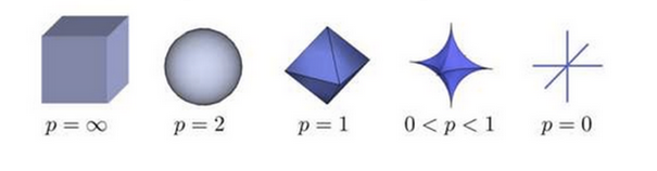 The above picture shows how the changes of the points whose distance (norm) to the origin is 1 in the three dimensional space.
L0 Norm
Normally we use L0 norm to represent the number of non-zero elements in a vector. Therefore, minimize L0 norm meams we want some weights become to zero, so that some features will not use in estimating, we can deduce the complexity of model through using L0 norm, unfortunately, it is hard to explain and calculate L0 norm since we can not interpret the meaning of zero-sqrt, and optimization of L0 norm is a NP hard question, but do not worry, we can use L1 norm to subtitue, which is an optimal convex approximation of L0 norm.
L1 Norm
This is the defination of L1 norm: \[||x||_1 = \sum_i{|x_i|}\] It represents the sum of the absolute values of non-zero elements in vector x. Due to the natural nature of L1 norm, the solution to L1 norm optimization is a sparse solution, we can use L1 norm to achieve the sparse of features, so that some unuseful features will be dropped.
L2 Norm
The defination of L2 norm is: \[||x||_2 = \sqrt{\sum_ix_i^2}\] We can make the value of weights toward to zero by minimizing L2 norm, but it is just toward instead of reaching at zero, which is different from L0 norm and L1 norm. Although there are several differences among L0, L1 and L2 norm, the essence of them is same, we use them to weaken or even drop some features, so that we can get a simpler model with a better generization ability.
How it works?
It is easy to answer this question after konwing the concept of norm: we just need to optimize the L1 or L2 norm, it can penalise weights atuomaticlly. However, do not forget our true aim: fitting data by minimizing the loss function. Therefore, we need to minimize loss function and regularization term simultaneously, but it is still easy to do that, we can minimize the sum of them: \[min{[R_{emp} + \lambda{r(w)}]}\] That is: \[min[{1\over{N}}\sum_{i=1}^NL(f(x_i), y_i) + {\lambda\over{2}}{||w||_2^2}]\] A larger lambda can impel to chose a simpler model and a smaller lambda will get a more complex model.
Why L1 is sparse and L2 is smooth?
As we said, L1 norm can make weights change to zero and L2 norm let the parameters toward to zero, we call L1 norm is sparse and L2 norm is smooth. We can understand this from different aspects.
Mathmatical Formula
Firstly, we assume the structural loss function with L1 norm is: \[L1 = R + {\lambda\over{n}}\sum_i|w_i|\] So we can calculate the derivative of w: \[{\partial{L1}\over{\partial{w}}}={\partial{R}\over{\partial{w}}}+{\lambda\over{n}}sign(w)\] And then: \[w^{t+1} = w^t - \eta{\partial{L1}\over{\partial{w^t}}}\] \[w^{t+1}=w^t-\eta{\partial{R}\over{\partial{w^t}}}-\eta{\lambda\over{n}}sign(w^t)\] And sign function is defined as: \[sign(x) = \begin{cases} +1 & x>0 \\ -1 & x<0 \\ [-1,1] & x=0 \end{cases}\] As for the structural risk function with L2 norm: \[L2 = R + {\lambda\over{2n}}\sum_iw_i^2\] And then: \[{\partial{L2}\over{\partial{w}}}={\partial{R}\over{\partial{w}}}+{\lambda\over{n}}w\] \[w^{t+1} = w^t - \eta{\partial{L2}\over{\partial{w^t}}}\] \[w^{t+1}=w^t-\eta{\partial{R}\over{\partial{w^t}}}-\eta{\lambda\over{n}}w^t\] \[w^{t+1}=(1-\eta{\lambda\over{n}})w^t-\eta{\partial{R}\over{\partial{w^t}}}\]
So we can see that the difference between the two formulas: the parameter w in \(L1\) minus \(\eta{\lambda\over{n}}sign(w)\) which is a constant for each \(w\) (see the deifnation of \(sign(x)\)). However, in \(L2\) it minus \(\eta{\lambda\over{n}}w\), which means \(w\) will reduce in a specific proportion in each iterations, and the proportion is \(\eta{\lambda\over{n}}\).
Therefore, in some extent, L1 norm can make the parameteres(\(w\)) reduce to zero since it minus a constant each time, and L2 norm makes the weights toward to zero because reducing with a specific proportion. This is also the reason why we can use L1 norm to do feature selection(automaticlly) and use L2 norm to make the parameters smaller, and we also call L2 norm as weight decay.
In addition, L2 norm has a more quicker reduction rate than L1 norm when \(w\) is in the interval \([1, +\infty]\), and L1 norm has a faster decreasing rate when \(w\) is in \((0, 1)\). So L1 norm can make \(w\) reach at zero more easier and get more zero elements in the parameter vector.
Geometric Space
We can also understand this question from geometric space.
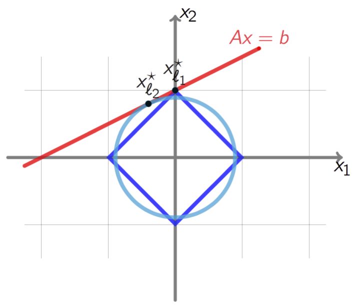 For the above picture, we assume that the red line is our empirical risk function(R), the light blue circle is the graph of L2 norm and the deep blue one is L1 norm. As we said, L1 and L2 norms are a kind of constraint for the function R, therefore, the intersection is our best solution, we can see that L1 norm can more easier to make the solution reach at zero.
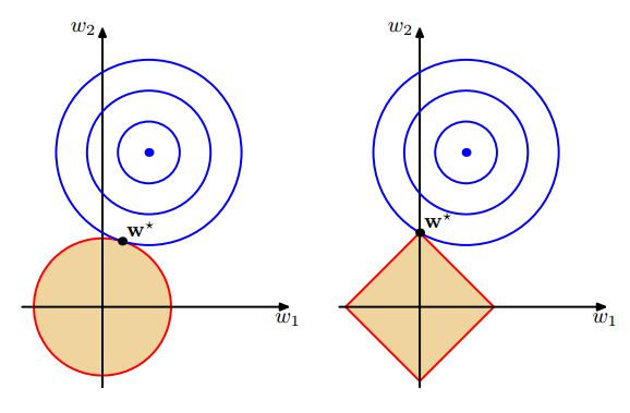
The same situation can be found in other empirical loss function, such as squared error:
I am going to introduce another interpretation in geometric space which I believe can help us to understand this question better.
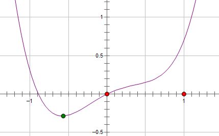 As the above graph shows, assume that the purple line is our empirical loss function (R), and the green point is the local minimum. Now, we add L2 norm to the function, so we can get \(R+\lambda x^2\):
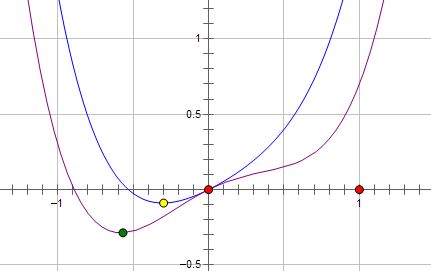 The minimun has changed to the yellow point, it can be seen that the optimum value has reduced, but is not zero. We can get the new function \(R+\lambda |x|\) with L1 norm:
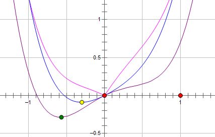 The optimum changed to zero (the pink line).
Remember that the truth is L1 norm can get optimum solution as zero more easier than L2 norm, which means we can not make sure the best value must be zero with L1 norm and L2 norm can also get zero value solution in the specific situation. I am going to interpret this situation.
Actually, whether the two norms can change the optimal solution (the parameter/weight) to zero is depend on the value of derivative of zero point (x=0) in the empirical loss function: the derivative of zero point can not change to zero so the optimal solution is also non-zero if the original function (R) has non-zero derivative in the point x=0, in other words, L2 norm can change the optimal value to zero if the derivative of \(R_{emp}\) is zero in x=0.
In terms of L1 norm, x=0 can be the optimal solution (local minimum) if the regularization coefficient \(\lambda\) is larger than the value of \(|R_{emp}'(0)|\) (since we need to guarantee the derivates of left side and right side of x=0 have the opposite sign): The derivative of left side: \[R_{emp}'(0)-\lambda\] The derivative of right side: \[R_{emp}'(0)+\lambda\] Therefore, if: \[\lambda \geq |R_{emp}'(0)|\] Then we can guarantee x=0 is the local minimum.